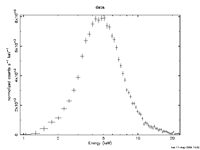
We shall start with a simple example based on very old data, an EXOSAT observation of GX301-2. First we read in the data :
                XSPEC version: 12.5.1
        Build Date/Time: Mon Aug  3 13:17:56 2009

XSPEC12>data file1.pha

1 spectrum  in use

Spectral Data File: file1.pha  Spectrum 1
Net count rate (cts/s) for Spectrum:1  3.586e+01 +/- 2.466e-01 (50.6 % total)
 Assigned to Data Group 1 and Plot Group 1
  Noticed Channels:  1-64
  Telescope: EXOSAT Instrument: ME  Channel Type: PHA
  Exposure Time: 2100 sec
 Using Background File                back1.pha
  Background Exposure Time: 3320 sec
 Using Response (RMF) File            resp1.rsp for Source
This dataset has associated background and response files which have been read in automatically because their names are given in file1.pha by the BACKFILE and RESPFILE keywords. If these keywords were not set, we could load the associated files using :
XSPEC12>back back1.pha
Net count rate (cts/s) for Spectrum:1  3.586e+01 +/- 2.466e-01 (50.6 % total)
XSPEC12>resp resp1.rsp
Response successfully loaded.
Generally the best first step is to look at the spectrum :
XSPEC12>cpd /xs
XSPEC12>plot data
XSPEC12>setp energy
XSPEC12>plot
The first command sets the plotting device to the X-window server. The third command switches the x-axis from channels to energy. If you want it in wavelength then use setp wave. Note that the plot command remembers the option from its last invocation.

This instrument had very little effective response at the ends of the range so we next remove some channels from consideration :
XSPEC12>ignore 1-3 45-**
     3 channels (1,3) ignored in spectrum #     1
    20 channels (45,64) ignored in spectrum #     1
Note that internally XSPEC always assumes that the first channel is number 1 (not 0). The ignore command can also be used to ignore channels over a specific energy range by giving the arguments as decimals :
XSPEC12>ig 0.-1.5 14.5-**
     3 channels (1-3) ignored in spectrum #     1
    20 channels (45-64) ignored in spectrum #     1
The opposite of ignore is notice, which uses the same syntax. We are now ready to define a model. XSPEC has over 100 available but presumably you have some physical understanding of the source which leads you to try particular models. Please do not randomly try all the models - that way lies madness. In this case a good choice is a power-law modified by photo-electric absorption due to intervening matter :
XSPEC12>model phabs(pow)

Input parameter value, delta, min, bot, top, and max values for ...
              1      0.001          0          0     100000      1e+06
1:phabs:nH>
              1       0.01         -3         -2          9         10
2:powerlaw:PhoIndex>
              1       0.01          0          0      1e+24      1e+24
3:powerlaw:norm>

========================================================================
Model phabs<1>*powerlaw<2> Source No.: 1   Active/On
Model Model Component  Parameter  Unit     Value
 par  comp
   1    1   phabs      nH         10^22    1.00000      +/-  0.0
   2    2   powerlaw   PhoIndex            1.00000      +/-  0.0
   3    2   powerlaw   norm                1.00000      +/-  0.0
________________________________________________________________________


 Chi-Squared =   1.742025e+07 using 40 PHA bins.
 Reduced chi-squared =       470817.6 for     37 degrees of freedom
 Null hypothesis probability =   0.000000e+00
 Current data and model not fit yet.
The model command prompts for starting parameter values. Entering <return> takes the default or you can give values that you think likely. Note that many places in XSPEC if you enter the special string /* you will be returned to the XSPEC12> prompt with appropriate defaults set. This is obviously not a good match to the data so we go ahead and let the fit algorithm try to find better values for the parameters :
XSPEC12>fit

Chi-Squared  Lvl Par #          1             2             3
718.634       -3    3.35171       0.578603      0.0253134
537.464       -2    5.52951       0.786511      0.0369648
315.366       -2    6.72975       0.93749       0.0518879
162.741       -2    7.46415       1.03946       0.0661236
107.665       -2    8.007         1.11228       0.0781108
85.6224       -2    8.41173       1.1657        0.0878649
75.3466       -2    8.71501       1.20519       0.0956644
71.4872       -3    9.3694        1.29233       0.113137
64.1984       -4    9.59685       1.31891       0.121118
64.0368       -5    9.61945       1.32064       0.121871
Number of trials exceeded: continue fitting?
After 10 iterations you will be prompted whether you want to continue. To change the number of iterations before a prompt just give the fit command an integer argument, eg fit 1000. Just hit <return> to continue :
64.0368       -6    9.62061       1.32071       0.121894
========================================
 Variances and Principal Axes
                 1        2        3
 4.6355E-07| -0.0055  -0.2015   0.9795
 9.3130E-02| -0.9946  -0.1003  -0.0263
 3.6427E-04| -0.1036   0.9743   0.1999
----------------------------------------

====================================
  Covariance Matrix
   1           2           3
9.213e-02   9.258e-03   2.426e-03
9.258e-03   1.284e-03   3.164e-04
2.426e-03   3.164e-04   7.929e-05
------------------------------------

========================================================================
Model phabs<1>*powerlaw<2> Source No.: 1   Active/On
Model Model Component  Parameter  Unit     Value
 par  comp
   1    1   phabs      nH         10^22    9.62061      +/-  0.303532
   2    2   powerlaw   PhoIndex            1.32071      +/-  3.58266E-02
   3    2   powerlaw   norm                0.121894     +/-  8.90457E-03
________________________________________________________________________


 Chi-Squared =          64.04 using 40 PHA bins.
 Reduced chi-squared =          1.731 for     37 degrees of freedom
 Null hypothesis probability =   3.792356e-03
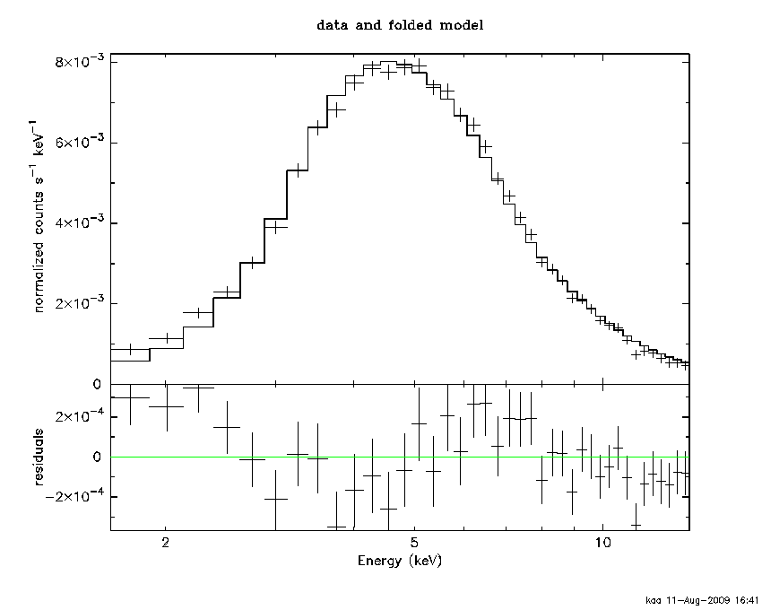
This is getting closer so let's look at the data, the model and the difference between them :

The residuals plot shows clear systematic trends so we don't have the model quite correct yet. The EXOSAT medium energy detector is a proportional counter with a rather poor resolution and we know that a fluorescent iron line may be detectable so let us try that :
XSPEC12>editmod phabs(pow+gauss)

Input parameter value, delta, min, bot, top, and max values for ...
            6.5       0.05          0          0      1e+06      1e+06
4:gaussian:LineE>6.4 0
            0.1       0.05          0          0         10         20
5:gaussian:Sigma>0 0
              1       0.01          0          0      1e+24      1e+24
6:gaussian:norm>1.0e-3

 Chi-Squared =          60.37 using 40 PHA bins.
 Reduced chi-squared =          1.677 for     36 degrees of freedom
 Null hypothesis probability =   6.661893e-03
 Current data and model not fit yet.

========================================================================
Model phabs<1>(powerlaw<2> + gaussian<3>) Source No.: 1   Active/On
Model Model Component  Parameter  Unit     Value
 par  comp
   1    1   phabs      nH         10^22    9.62061      +/-  0.303532
   2    2   powerlaw   PhoIndex            1.32071      +/-  3.58266E-02
   3    2   powerlaw   norm                0.121894     +/-  8.90457E-03
   4    3   gaussian   LineE      keV      6.40000      frozen
   5    3   gaussian   Sigma      keV      0.0          frozen
   6    3   gaussian   norm                1.00000E-03  +/-  0.0

________________________________________________________________________
The editmod command allows us to add a single model component and prompts for its starting parameter values. By entering two numbers for line energy we set the starting value to 6.4 keV and fix its value. Entering a 0 after the parameter value acts as a switch changing the status of the parameter from variable (thawed) to fixed (frozen) or vice versa. We froze the line width to zero because the data will not constrain it and picked a normalization which will be roughly correct :
XSPEC12>fit 100

Chi-Squared  Lvl Par #          1             2             3             6
50.7699       -3    9.30187       1.31308       0.11659       0.0011305
50.7038       -4    9.24659       1.30706       0.11512       0.00103439
50.689        -5    9.24138       1.30663       0.115013      0.00111476
50.6788       -6    9.24031       1.30653       0.114988      0.00105047
50.6728       -7    9.24051       1.30655       0.114993      0.00110209
==================================================
 Variances and Principal Axes
                 1        2        3        6
 1.3411E-07| -0.0015  -0.0804   0.3938   0.9157
 7.4253E-07|  0.0065   0.1641  -0.9009   0.4018
 9.8299E-02|  0.9950   0.0966   0.0246  -0.0004
 4.0875E-04| -0.0995   0.9784   0.1810   0.0079
--------------------------------------------------

================================================
  Covariance Matrix
   1           2           3           4
9.733e-02   9.408e-03   2.397e-03   -4.401e-05
9.408e-03   1.309e-03   3.057e-04   -1.052e-06
2.397e-03   3.057e-04   7.343e-05   -7.170e-07
-4.401e-05  -1.052e-06  -7.170e-07  2.773e-07
------------------------------------------------

========================================================================
Model phabs<1>(powerlaw<2> + gaussian<3>) Source No.: 1   Active/On
Model Model Component  Parameter  Unit     Value
 par  comp
   1    1   phabs      nH         10^22    9.24051      +/-  0.311971
   2    2   powerlaw   PhoIndex            1.30655      +/-  3.61737E-02
   3    2   powerlaw   norm                0.114993     +/-  8.56921E-03
   4    3   gaussian   LineE      keV      6.40000      frozen
   5    3   gaussian   Sigma      keV      0.0          frozen
   6    3   gaussian   norm                1.10209E-03  +/-  5.26630E-04
________________________________________________________________________


 Chi-Squared =          50.67 using 40 PHA bins.
 Reduced chi-squared =          1.408 for     36 degrees of freedom
 Null hypothesis probability =   5.322983e-02
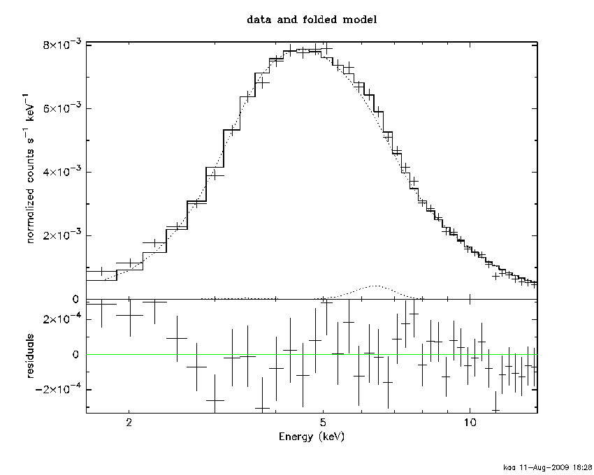
XSPEC12>setp add
XSPEC12>pl

The setp add command ensures that all subsequent data plots will show individual additive model components. This option can be turned off again by setp noadd. The fit is not perfect yet although the residuals are at the low energy end where we might be a bit suspicious about the calibration.
