The advantage of surveying external galaxies with a significant supernova
rate is that we can translate our results into estimates of abundances and
rates. We scale our rates using the observed supernova rate of
![]() year
year![]() (
(
![]() at 90% confidence).
As we discussed in PaperI, this is significantly higher than standard star
formation rate estimates for these galaxies, but the SN rate is directly
proportional to the massive star formation rate rather than an indirect
indicator, and similar discrepancies, although not as dramatic, have been
noted in other contexts (e.g., Horiuchi et al.2011).
In this section we first outline how we will
estimate rates, and then we discuss the constraints on analogs of
at 90% confidence).
As we discussed in PaperI, this is significantly higher than standard star
formation rate estimates for these galaxies, but the SN rate is directly
proportional to the massive star formation rate rather than an indirect
indicator, and similar discrepancies, although not as dramatic, have been
noted in other contexts (e.g., Horiuchi et al.2011).
In this section we first outline how we will
estimate rates, and then we discuss the constraints on analogs of ![]() Car
and the implications of our sample of luminous dusty stars.
Car
and the implications of our sample of luminous dusty stars.
We are comparing a sample of ![]() supernovae observed over
supernovae observed over ![]() years
to a sample of
years
to a sample of ![]() candidate stars which are detectable by our selection procedures
for a time
candidate stars which are detectable by our selection procedures
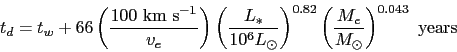
for a time ![]() . In PaperI we used DUSTY to model the detection of expanding
dusty shells and found that a good estimate for the detection time period was
. In PaperI we used DUSTY to model the detection of expanding
dusty shells and found that a good estimate for the detection time period was
 |
(5) |
The transient rate in a sample of galaxies is less interesting than comparing the rate
to the supernova rate. Let ![]() be the fraction of massive (
be the fraction of massive (
![]() ) stars that
create the transients, where
) stars that
create the transients, where
![]() if we
assume a Salpeter IMF (Kennicutt1998), that all stars more massive than
if we
assume a Salpeter IMF (Kennicutt1998), that all stars more massive than ![]() become
supernovae and that all stars more massive than
become
supernovae and that all stars more massive than ![]() cause the transients.
If each star undergoes an average of
cause the transients.
If each star undergoes an average of ![]() eruptions, then the rate of transients is related
to the rate of supernovae by
eruptions, then the rate of transients is related
to the rate of supernovae by
![]() . The
interesting quantity to constrain is
. The
interesting quantity to constrain is ![]() rather than
rather than ![]() . Poisson
statistics provide constraints on the rates,
where
. Poisson
statistics provide constraints on the rates,
where
![]() for
for ![]() events observed over a time
period
events observed over a time
period ![]() . This means that the probability of the rates given the data is
. This means that the probability of the rates given the data is
| (6) |
| (7) |