


Next: About this document ...
Up: Finding Car Analogs in
Previous: Conclusions
-
Abazajian, K. N. et al. 2009, , 182, 543
-
-
Alard, C. 2000, , 144, 363
-
-
Alard, C. & Lupton, R. H. 1998, , 503, 325
-
-
Balog, Z. et al. 2013, Experimental Astronomy
-
-
Bionta, R. M., Blewitt, G., Bratton, C. B., Casper, D., & Ciocio, A.
1987, Physical Review Letters, 58, 1494
-
-
Chevalier, R. A. & Fransson, C. 1994, , 420, 268
-
-
Chugai, N. N. & Danziger, I. J. 2003, Astronomy Letters, 29, 649
-
-
Cox, P., Mezger, P. G., Sievers, A., Najarro, F., Bronfman, L.,
Kreysa, E., & Haslam, G. 1995, , 297, 168
-
-
Cutri, R. M. et al. 2003, 2MASS All Sky Catalog of point sources., ed.
R. M. Cutri et al.
-
-
Dalcanton, J. J. et al. 2009, , 183, 67
-
-
Dale, D. A. et al. 2009, ApJ, 703, 517
-
-
Davidson, K. 1987, , 317, 760
-
-
de Jager, C. 1998, , 8, 145
-
-
de Jager, C. & Nieuwenhuijzen, H. 1997, , 290, L50
-
-
Dolphin, A. E. 2000, , 112, 1383
-
-
Draine, B. T. & Lee, H. M. 1984, , 285, 89
-
-
Egan, M. P., Clark, J. S., Mizuno, D. R., Carey, S. J., Steele,
I. A., & Price, S. D. 2002, , 572, 288
-
-
Elitzur, M. & Ivezic, Z. 2001, , 327, 403
-
-
Fazio, G. G. et al. 2004, , 154, 10
-
-
Figer, D. F., McLean, I. S., & Morris, M. 1999, , 514, 202
-
-
Filippenko, A. V. 1997, , 35, 309
-
-
Fullerton, A. W., Massa, D. L., & Prinja, R. K. 2006, , 637, 1025
-
-
Gal-Yam, A. et al. 2007, , 656, 372
-
-
Gal-Yam, A., & Leonard, D. C. 2009, , 458, 865
-
-
Gardner, J. P. et al. 2006, , 123, 485
-
-
Gerke, J. R., Kochanek, C. S., Prieto, J. L., Stanek, K. Z., &
Macri, L. M. 2011, , 743, 176
-
-
GSC2.2. 2001, VizieR Online Data Catalog, 1271, 0
-
-
Gvaramadze, V. V., Kniazev, A. Y., & Fabrika, S. 2010, , 405, 1047
-
-
Heger, A., Fryer, C. L., Woosley, S. E., Langer, N., & Hartmann,
D. H. 2003, , 591, 288
-
-
Higgs, L. A., Wendker, H. J., & Landecker, T. L. 1994, , 291, 295
-
-
Horiuchi, S., Beacom, J. F., Kochanek, C. S., Prieto, J. L., Stanek,
K. Z., & Thompson, T. A. 2011, , 738, 154
-
-
Hubble, E. & Sandage, A. 1953, , 118, 353
-
-
--. 1984, Science, 223, 243
-
-
Humphreys, R. M. & Davidson, K. 1994, PASP, 106, 1025
-
-
Humphreys, R. M., Jones, T. J., & Gehrz, R. D. 1987, , 94, 315
-
-
Humphreys, R. M., Davidson, K., & Smith, N. 1999, , 111, 1124
-
-
--. 2002, , 124, 1026
-
-
Humphreys, R. M. et al. 1997, , 114, 2778
-
-
Humphreys, R. M., Davidson, K., Jones, T. J., Pogge, R. W., Grammer,
S. H., Prieto, J. L., & Pritchard, T. A. 2012, , 760, 93
-
-
--. 2006, AJ, 131, 2105
-
-
Ivezic, Z. & Elitzur, M. 1997, , 287, 799
-
-
Ivezic, Z., Nenkova, M., & Elitzur, M. 1999, ArXiv Astrophysics
e-prints, 9910475
-
-
Jones, T. J. et al. 1993, , 411, 323
-
-
Kennicutt, Jr., R. C. et al. 2003, PASP, 115, 928
-
-
Khan, R., Stanek, K. Z., & Kochanek, C. S. 2013, , 767, 52
-
-
Khan, R., Stanek, K. Z., Kochanek, C. S., & Bonanos, A. Z. 2011, ,
732, 43
-
-
Khan, R., Stanek, K. Z., Prieto, J. L., Kochanek, C. S., Thompson,
T. A., & Beacom, J. F. 2010, ApJ, 715, 1094
-
-
Kennicutt, Jr., R. C. 1998, , 498, 541
-
-
Kochanek, C. S. 2011, , 743, 73
-
-
Kochanek, C. S., Szczygie
 , D. M., & Stanek, K. Z. 2012, , 758,
142
, D. M., & Stanek, K. Z. 2012, , 758,
142
-
-
Kochanek, C. S. et al. 2008, , 684, 1336
-
-
Kourniotis, M. et al. 2014, , 562, A125
-
-
Kozlowski, S., Kochanek, C. S., Stern, D., Prieto, J. L., & Stanek,
K. Z. 2010, Central Bureau Electronic Telegrams, 2392, 1
-
-
Liu, J. 2011, , 192, 10
-
-
Maeder, A. 1981, , 101, 385
-
-
Maeder, A. & Meynet, G. 1987, , 182, 243
-
-
--. 1988, , 76, 411
-
-
Massey, P., Olsen, K. A. G., Hodge, P. W., Strong, S. B., Jacoby,
G. H., Schlingman, W., & Smith, R. C. 2006, AJ, 131, 2478
-
-
Mauerhan, J. C. et al. 2013, , 430, 1801
-
-
McQuinn, K. B. W. et al. 2007, ApJ, 664, 850
-
-
Meynet, G., Maeder, A., Schaller, G., Schaerer, D., & Charbonnel, C.
1994, , 103, 97
-
-
Mineo, S., Gilfanov, M., & Sunyaev, R. 2012, , 419, 2095
-
-
Moriya, T. J., Maeda, K., Taddia, F., Sollerman, J., Blinnikov,
S. I., & Sorokina, E. I. 2014, , 439, 2917
-
-
Nieuwenhuijzen, H. & de Jager, C. 2000, , 353, 163
-
-
Ochsenbein, F., Bauer, P., & Marcout, J. 2000, , 143, 23
-
-
Ofek, E. O. et al. 2013, , 494, 65
-
-
--. 2014a, , 789, 104
-
-
--. 2014b, , 781, 42
-
-
Ott, C. D. 2009, Classical and Quantum Gravity, 26, 204015
-
-
Pastorello, A. et al. 2007, , 447, 829
-
-
--. 2013, , 767, 1
-
-
Poglitsch, A. et al. 2010, , 518, L2
-
-
Prieto, J. L., Brimacombe, J., Drake, A. J., & Howerton, S. 2013,
, 763, L27
-
-
Remillard, R. A. & McClintock, J. E. 2006, , 44, 49
-
-
Rieke, G. H. et al. 2004, , 154, 25
-
-
Robinson, G., Hyland, A. R., & Thomas, J. A. 1973, , 161, 281
-
-
Schlegel, E. M. 1990, , 244, 269
-
-
Smartt, S. J. 2009, , 47, 63
-
-
Smith, N. 2009, ArXiv e-prints, 0906.2204
-
-
--. 2014, ArXiv e-prints
-
-
Smith, N. & McCray, R. 2007, , 671, L17
-
-
Smith, N. & Owocki, S. P. 2006, , 645, L45
-
-
Smith, N., Vink, J. S., & de Koter, A. 2004, , 615, 475
-
-
Smith, N. 2006, , 644, 1151
-
-
Smith, N. et al. 2008, , 686, 467
-
-
Smith, N., Li, W., Silverman, J. M., Ganeshalingam, M., &
Filippenko, A. V. 2011, , 415, 773
-
-
Stanek, K. Z. et al. 2003, , 591, L17
-
-
Stoll, R. et al. 2011, , 730, 34
-
-
Stothers, R. B. & Chin, C.-W. 1996, , 468, 842
-
-
Szczygie, D. M., Gerke, J. R., Kochanek, C. S., & Stanek, K. Z.
2012, , 747, 23
-
-
Tiffany, C., Humphreys, R. M., Jones, T. J., & Davidson, K. 2010, ,
140, 339
-
-
Ueta, T., Meixner, M., Dayal, A., Deutsch, L. K., Fazio, G. G.,
Hora, J. L., & Hoffmann, W. F. 2001, , 548, 1020
-
-
Vink, J. S., Davies, B., Harries, T. J., Oudmaijer, R. D., &
Walborn, N. R. 2009, , 505, 743
-
-
Voors, R. H. M. et al. 2000, , 356, 501
-
-
Wachter, S., Mauerhan, J. C., Van Dyk, S. D., Hoard, D. W., Kafka,
S., & Morris, P. W. 2010, , 139, 2330
-
-
Woods, P. M. et al. 2011, , 411, 1597
-
-
Wright, E. L. et al. 2010, , 140, 1868
-
Figure 1:
The spectral energy distributions (SEDs) of the dust-obscured massive
star  Car (dash-dot line, e.g., Robinson et al.1973; Humphreys & Davidson1994),
``ObjectX'' in M33 (dashed line; Khan et al.2011), and
an obscured star in M81 that we identify in this paper
(M81-12, solid line). All these stars have SEDs that
are flat or rising in the Spitzer IRAC 3.6, 4.5, 5.8 and
Car (dash-dot line, e.g., Robinson et al.1973; Humphreys & Davidson1994),
``ObjectX'' in M33 (dashed line; Khan et al.2011), and
an obscured star in M81 that we identify in this paper
(M81-12, solid line). All these stars have SEDs that
are flat or rising in the Spitzer IRAC 3.6, 4.5, 5.8 and  bands (marked here by solid circles).
The three shortest wavelength data-points of the M81-12 SED are from HST
bands (marked here by solid circles).
The three shortest wavelength data-points of the M81-12 SED are from HST  images.
The
images.
The  measurements of both ObjectX and M81-12 are from
Spitzer MIPS while the dotted segments of their SEDs show the
Herschel PACS 70, 100, and
measurements of both ObjectX and M81-12 are from
Spitzer MIPS while the dotted segments of their SEDs show the
Herschel PACS 70, 100, and  upper limits.
|
Figure:
The Hubble, Spitzer, and
Herschel images of the region around M81-12.
In the left panel, the radii of the circles are  (5 ACS pixels) and
  (IRAC
(IRAC
 PSF FWHM), and the source at the position of the
smaller circle in the left panel is the brightest red point
source on the CMD (Figure4, left panel).
The red line in each panel is the size of a
PACS pixel (
PSF FWHM), and the source at the position of the
smaller circle in the left panel is the brightest red point
source on the CMD (Figure4, left panel).
The red line in each panel is the size of a
PACS pixel ( ).
).
|
Figure:
The Spitzer MIPS 24, 70 and (top row)
and Herschel PACS 70, 100 and (bottom row) images
of the region around the object N7793-9. The higher resolution of the
PACS images helps us set tighter limits on the far-IR emission from
the candidates.
|
Figure 4:
The  (
( ) vs.
) vs.  (
( ) color magnitude diagram (CMD) for all HST point
sources around M81-12. The three large solid triangles denote sources located with the
) color magnitude diagram (CMD) for all HST point
sources around M81-12. The three large solid triangles denote sources located with the
 matching radius. The small open triangles show all other sources within
a larger
matching radius. The small open triangles show all other sources within
a larger  radius to emphasize the absence
of any other remarkable sources nearby.
The circle marks the source at the position of the
smaller circle in the left panel of Figure2,
which is the brightest red point source on the CMD.
The excellent (
radius to emphasize the absence
of any other remarkable sources nearby.
The circle marks the source at the position of the
smaller circle in the left panel of Figure2,
which is the brightest red point source on the CMD.
The excellent ( ) astrometric
match and the prior that very red sources are rare
confirms that this source is the optical counterpart of the
mid-IR bright red Spitzer source.
) astrometric
match and the prior that very red sources are rare
confirms that this source is the optical counterpart of the
mid-IR bright red Spitzer source.
|
Figure 5:
The differential light curves of some of
the candidates in M81 and NGC2403 obtained from
the Large Binocular Telescope.
The data spans the period from March2008 to
January2013. The  (squares),
  (triangles),
(circles),
(triangles),
(circles),  (crosses) differential magnitudes
are offset by
(crosses) differential magnitudes
are offset by
 mag for clarity.
|
Figure 6:
The best fit model (solid line)
of the observed SED (squares and triangles, the latter show
flux upper limits) of M81-12
and the SED of the
underlying, unobscured star (dashed line),
as compared to
Car (dotted line).
The best fit is for a
 ,
,
 star
obscured by
star
obscured by  ,
,
 silicate dust
shell at
silicate dust
shell at
 cm.
cm.
|
Figure 7:
Same as Figure6, but showing all the obscured
stars that we identified as compared to M33VarA,  , and
Car. The solid line shows the best fit model of the observed SED,
and the dashed line shows the SED of the
underlying, unobscured star. M33VarA and are shown on
separate panel while Car is shown on every panel (dotted line).
, and
Car. The solid line shows the best fit model of the observed SED,
and the dashed line shows the SED of the
underlying, unobscured star. M33VarA and are shown on
separate panel while Car is shown on every panel (dotted line).
|
Figure 8:
The SEDs of the 16 candidates that we concluded are not stars
(points and solid lines) as compared to Car (dotted line).
|
Figure:
Luminosities of the obscured stars
as a function of the estimated ejecta mass determined
from the best fit model for each SED.
The dashed lines enclose the luminosity range
 .
We do not show N7793-3 for which we have no optical or near-IR data.
(square), M33VarA (triangle), and Car (star symbol)
are shown for comparison. The error bar
corresponds to the typical
.
We do not show N7793-3 for which we have no optical or near-IR data.
(square), M33VarA (triangle), and Car (star symbol)
are shown for comparison. The error bar
corresponds to the typical  uncertainties on
  (
( )
and
)
and  (
( ) of the best SED fit models.
|
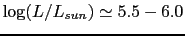
Figure 10:
Same as Figure9, but for different dust types and
temperature assumptions. The top row shows the best silicate (left), graphitic (center),
and the better of the two (right, same as Figure9) models.
The middle and bottom rows show the best fit models for graphitic
and silicate dust at fixed stellar temperatures of 5000K, 7500K and 20000K.
The only higher luminosity case in the fixed temperature model panels is N2403-4,
for which the best fit models have significantly smaller  and lower luminosities
for both dust types.
and lower luminosities
for both dust types.
|
Figure 11:
Cumulative histograms of the dust shell radius  for the newly identified stars
excluding N7793-3. The dotted lines, normalized to the point where
for the newly identified stars
excluding N7793-3. The dotted lines, normalized to the point where
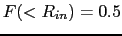 , shows the distribution expected for shells in
uniform expansion observed at a random time.
, shows the distribution expected for shells in
uniform expansion observed at a random time.
|
Figure 12:
Elapsed time
 as a function of the estimated ejecta mass
for the best fit graphitic models.
The mass and radius are scaled to
as a function of the estimated ejecta mass
for the best fit graphitic models.
The mass and radius are scaled to
 cm
cm gm
gm and
and
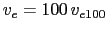 kms, and
can be rescaled as
kms, and
can be rescaled as
 and
and
 .
The error bar shows the typical uncertainties on
.
The error bar shows the typical uncertainties on  (
( )
and () of the best SED fit models..
The three dotted lines correspond to optical depths
)
and () of the best SED fit models..
The three dotted lines correspond to optical depths
 and
and  .
We should have trouble finding sources with
.
We should have trouble finding sources with  due to
lack of mid-IR emission and
due to
lack of mid-IR emission and
 due to
the dust photosphere being too cold (peak emission in far-IR).
The large estimate for Car when
scaled by
due to
the dust photosphere being too cold (peak emission in far-IR).
The large estimate for Car when
scaled by  is due to the anomalously
large ejecta velocities (
is due to the anomalously
large ejecta velocities ( kms along the
long axis (Smith2006; Cox et al.1995) compared to
typical LBV shells (
kms along the
long axis (Smith2006; Cox et al.1995) compared to
typical LBV shells ( kms, Tiffany et al.2010).
|
Table 1:
PACS Aperture Definitions
Band ( ) ) |
Pixel Scale |
 |
|
 |
Ap. Corr. |
| |
|
|
|
|
|
 |
|
 |
 |
 |
 |
 |
|
|
|
|
 |
|
|
 |
 |
 |
 |
| |
|
|
|
|
|
![\begin{landscape}
% latex2html id marker 1129\begin{table*}[p]
\begin{center}
...
...rent magnitudes, not \textit{Herschel} flux (mJy).}
\end{table*}\end{landscape}](img266.png)
![\begin{landscape}
% latex2html id marker 1212\begin{table*}[p]
\begin{center}
...
...ne
\hline
\end{tabular}
\end{tiny}
\end{center}
\end{table*}\end{landscape}](img267.png)
![\begin{landscape}
% latex2html id marker 1342\begin{table*}[p]
\begin{center}
...
...ne
\hline
\end{tabular}
\end{tiny}
\end{center}
\end{table*}\end{landscape}](img268.png)
![\begin{landscape}
% latex2html id marker 1475\begin{table*}[p]
\begin{center}
...
...ne
\hline
\end{tabular}
\end{tiny}
\end{center}
\end{table*}\end{landscape}](img269.png)
Next: About this document ...
Up: Finding Car Analogs in
Previous: Conclusions
Rubab Khan
2014-10-23
![\includegraphics[angle=0,width=130mm]{Eta_sed.ps}](img235.png)
![\includegraphics[angle=0,width=150mm]{m81-12_all.ps}](img238.png)
![\includegraphics[angle=0,width=150mm]{mips_pacs.ps}](img243.png)
![\includegraphics[angle=0,width=130mm]{cmd12a.ps}](img244.png)
![\includegraphics[angle=0,width=165mm]{LC.ps}](img245.png)
![\includegraphics[angle=0,width=130mm]{Dusty2.ps}](img246.png)
![\includegraphics[angle=0,width=165mm]{accept.ps}](img247.png)
![\includegraphics[angle=0,width=140mm]{reject.ps}](img248.png)
![\includegraphics[angle=0,width=130mm]{HR_like.ps}](img249.png)
![\includegraphics[angle=0,width=160mm]{Dusty.ps}](img251.png)
![\includegraphics[angle=0,width=130mm]{complete.ps}](img252.png)
![\includegraphics[angle=0,width=130mm]{TV.ps}](img253.png)