1.     GALEX Surveys and Sensitivities.

2.     Data Collection Modes.

3.     GALEX Photometric Properties.

4.     GALEX Imaging Bands --- Relation to other instrument bandpasses.

5.     GALEX Spectroscopic Properties.

6.     GALEX Astrometric Properties and Performance.

 

1.                GALEX Surveys and Sensitivities

The GALEX mission consists of  a series of nested imaging and spectroscopic surveys.  These surveys are performed concurrently---observations for each survey type are scheduled based on target availability.  Table 2.1 describes the primary GALEX surveys, the minimum exposure time, limiting magnitudes and science goals and objectives. 

 

Table 2.1 --  Primary Science Survey Summary

Survey	Survey Parameters			Science Objective			<z>
	Area [deg2]	Length [Month]	Expos [ksec]	Mag. Lim [mAB]	#Gals (est.)	Volume [Gpc3]
All-sky (AIS)	40,000	4	0.1	20.5	107	1.5	0.2
Wide Spectroscopic (WSS)	80	4	30	20	104-5	0.03	0.15
Nearby Galaxies (NGS)	---	0.5	1.5	27.5 [mag arcsec-2]	100	---	--
Medium Imaging (MIS)	1000	2	1.5	23	3 x 106	~1	0.6
Medium Spectroscopic (MSS)	8	2	300	21.5[R=100] 23.3[R=20]	104-5	0.03	0.5
Deep Spectroscopic (DSS)	2	4	1500	22.5[R=100] 24.3[R=20]	104-5	0.05	0.9
Deep Imaging (DIS)	80	4	30	25	107	1.0	0.85
Ultra-Deep Imaging (UDIS)	4	1	150	26	3x105	0.05	0.9

 

 

 

 

 

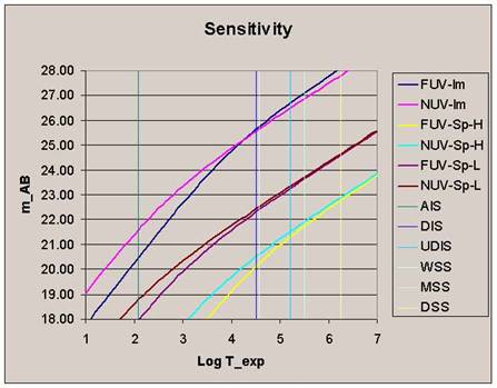Sensitivity vs. exposure time for low background targets (DIS, which have low diffuse galactic light and zodiacal background) is shown in Figure 1.1.  At these background levels, imaging surveys are background limited for exposures longer than 2 ksec [NUV] and 10 ksec [FUV] respectively.  Background levels may be as high as 3-5 times these, with corresponding reduction in the transitional exposure time.  Baseline survey sensitivities (typically specified as 5 sigma for imaging and 10 sigma for spectroscopy) are given in Table 2.1.

 

 

 

 

 

 

 

 

 

 

 

 

2.                Data Collection Modes

GALEX performs its surveys with plans that employ a simple operational scheme requiring only two observational modes and two instrument configurations.  Each orbit GALEX collects data during night segments (eclipses) of its orbits during visits to a single pre-programmed target. Each target consists either of a single pointing (single visit observation) or multiple adjacent pointings (sub-visit observations).   Currently sub-visits are only used for all-sky imaging survey (AIS) and in-flight calibration observations. The two instrument modes used for astronomical observations are imaging (aka direct) and grism. Only one optics wheel configuration is only set once per visi.  After removing instrument overhead, each eclipse typically yields up to 1700 seconds of usable science data.  Some observations are shortened by SAA passages when the detector high voltage must be kept at a safe, low level.

During any visit or sub-visit observation the spacecraft attitude is controlled in a tight, spiraled dither. A spiral dither is used to prevent “burn-in” of the detector active area by bright objects and to average over high spatial frequency response variations.  For each sub-visit the spiral dither pattern is restarted. Since celestial sources will move on the detector, the pipeline software will reposition the time-tagged photons to common sky coordinates based on the satellite aspect solution.

 

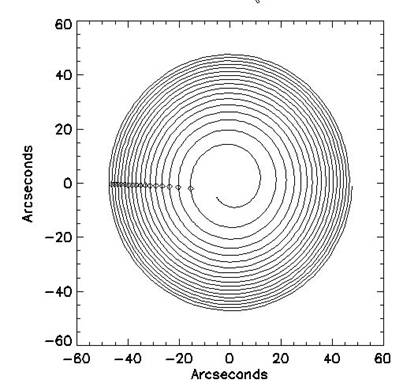
GALEX Dither spiral pattern during a 2100 second observation.  Diamonds are spaced every 120 seconds (1 revolution every two minutes).  The GALEX dither is a controlled spiral motion of the satellite that moves the telescope boresite in a tight, slow spiral pattern that moves outward to ~1.5' diameter across the sky.  This motion is used for all targeted observations.  The dither spiral has the following angular rate profile:

     

 

 

As many as 12 sub-visits are allowed per eclipse period (typical for AIS), with all-sky survey sub-visits obtaining 100-110 s exposure time per leg.  For plans with sub-visit targets, a 20 second slew time is required to move between each leg of the observation.  For some survey plans (e.g. deep imaging, spectroscopy), a single visit is insufficient to build up the requisite signal-to-noise, so a series of visits are needed in order to obtain the minimum required exposure time.

 

                                         

Table 1 .2 Sample observation Summary

 

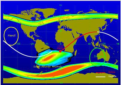Figure above shows time-series plots for a set of observations described in Table 1.2.  The top horizontal line in red, green and orange, indicates eclipse, day and SAA periods respectively.  The 4^th and 5^th rows plot the NUV and FUV detector count rate vs. time.  All-sky survey (sub-visit) eclipses 3023 and 3024 show discrete jumps in count rate throughout.  Eclipses 3025 and 3026 are single pointing visits.  For these observations the smooth variation in count rate vs. time is due to diffuse residual airglow background (predominantly a function of zenith angle).

The plot to the right is a satellite ground trace for eclipse 3027 (red ­ night; white ­ day). Because the satellite begins the eclipse inside the South Atlantic Anomaly the total exposure time is shorter than the maximum possible.

 

 

           

 

 

 

3.                GALEX Photometric Properties

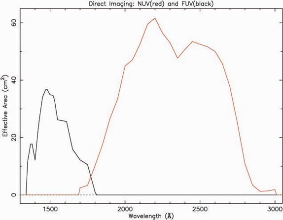
Figure 2 .1­ Effective area vs. wavelength for imaging mode.

 

Basic properties of the FUV and NUV bands are given in table below.  GALEX zero-points have been determined for the passband measured during ground calibration and will be refined based on in-flight measurements of spectrophotometric standards.  Current estimates are that the zero-points are accurate to within +/-10% (1 sigma).

 

Table 1.1 ­  GALEX Imaging Bands

Parameter	Description	Fuv	Nuv	Units
	effective wavelength	1516	2267	Å
	Pivot wavelength	1524	2297	Å
	Average wavelength	1529	2312	Å
	rms bandwidth	114	262	Å
	FWHM bandwidth	269	616	Å
	effective bandwidth	268	732	Å
Uresp	unit response (1 cps; mGALEX = 0)			erg s-1 cm-2 Å-1
f0	fGALEX  (1 cps;  mGALEX = 0)	108	36
m0 (AB)	mAB-mGALEX	18.82	20.08	Magnitudes
m0 (STLAM)	mSTLAM-mGALEX	16.04	18.18	Magnitudes
m0 (AB) ­ m0 (STLAM)	mAB-mSTLAM	2.78	1.90	Magnitudes

 

 

Unless designated as “calibrated” the GALEX magnitude is defined as:

 

 

where cps is the counts per second and rr is the relative response (~1) at the field position of the object.

GALEX “calibrated” (broadband) magnitudes are converted to a system with AB zero-point:

 

 

4.                  GALEX Imaging Bands --- Relation to other instrument bandpasses

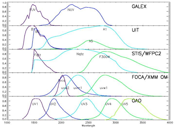
Figure 3 GALEX FUV and NUV shown in relation to bandpasses from other missions.  All are in normalized units (with the exception of UIT)

 

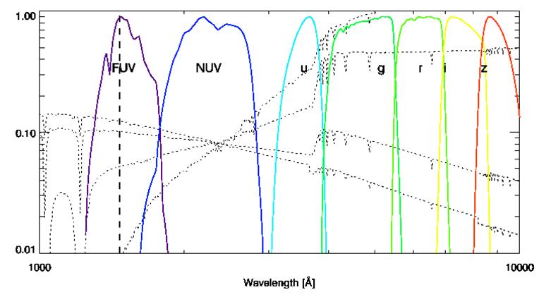
Figure 4 GALEX FUV and NUV shown in relation to SDSS bands.  (Dashed) Spectra for galaxies with varying burst history (young to old)

 

 

5.                GALEX Spectroscopic Properties

 

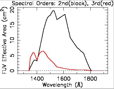
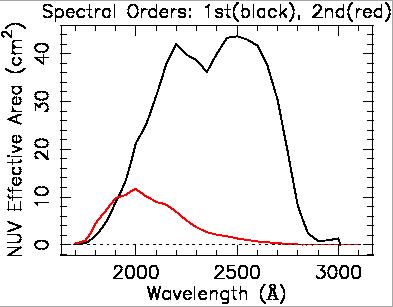
Figure 5 - Effective area vs. wavelength for FUV (left) and NUV (right) grism mode, 1st, 2nd, 3rd order

 

 

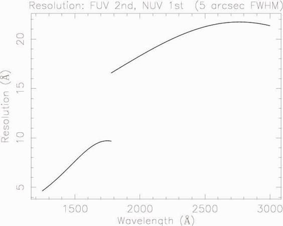
Figure 6 - Spectral Resolutiomn vs. Wavelength for FUV (2nd order, left) and NUV (1st order, right) grism mode.

 

 

 

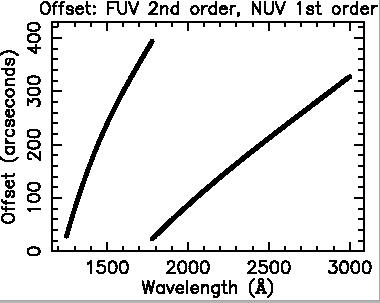
Figure 7 Spectral Dispersion vs. Wavelength (primary order)

 

 

6.                GALEX Astrometric Properties and Performance

 

GALEX images and catalogs are tied to the Tycho-2 frame using star positions from the ACT catalog.  Relative and absolute astrometric correction of satellite motion is performed in short (1-5 s) time intervals using stars measured by the NUV detector.  This results in refined aspect solution which is used to determine where each time-tagged photon originated in the sky for both  the NUV and FUV detectors.

 

Because GALEX records time-tagged photon positions with digitization that oversamples the instrumental PSF (x3-5) the pipeline map accumulator can rebin photon positions onto an idealized projection.  Sky images are generated using a gnomonic projection onto the tangent plane.   All output images contain standard FITS WCS astrometric header information.  Currently, intensity and count maps contain 3840 x 3840 with 1.5”x1.5” pixels.

 

Once in-flight calibration is complete, we expect that GALEX images will have no additional distortion component other than random small  (<0.5”) offsets.  Current pipeline performance is yielding a median offset in radius of 1.0” with an offset <2.4” for 90% of detected stellar sources.

 

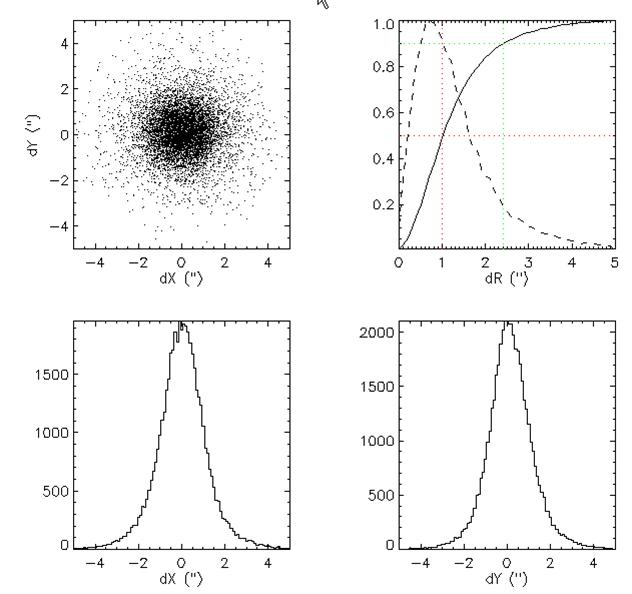
Figure 1.4­ Astrometric performance compared to known star positions. Panels: upper left—scatter plot. upper right—1D radial offset cumulative and density distribution. Lower left—distribution of offset in X (RA) and Y (dec) directions.