Results: Gravitational waves from Sgr A*!?

Our simulations cover 20Gyrs. Over this time scale, the nucleus model experiences a relatively important evolution. Most notably, significant relaxational mass segregation occurs, as Fig. 1 testifies.

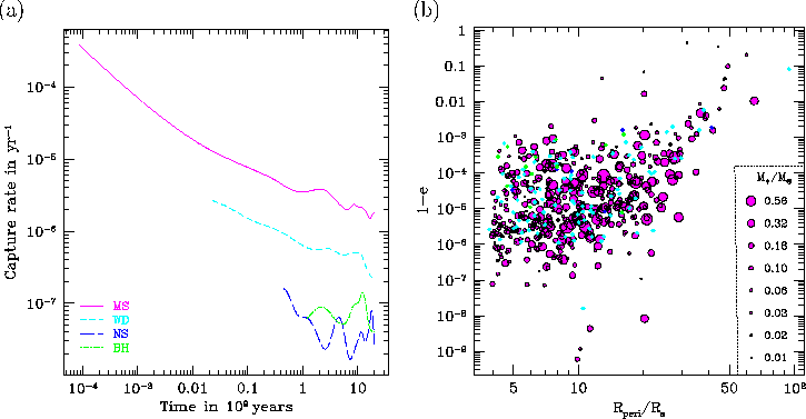
Fig. 2 shows the evolution of the capture rates as well as the orbital parameters at captures.

Figure 1: Mass-segregation due to 2-body Relaxation in our simulation of the Galactic centre. (a): evolution of the Lagrangian radii, i.e. the radii of spheres containing the indicated fraction of the total mass of the various stellar species: MS stars, white dwarfs (WD), neutron stars (NS) and stellar BHs (BH). (b): Density profiles at the end of the simulation ($T=24$Gyrs).

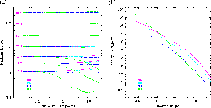Figure 2: Captures through emission of gravitational waves for our simulation of the Galactic centre. (a): Evolution of the capture rates for the various stellar species is shown. Note that only a small number of events have occurred for stellar BHs or NSs, hence the noisy curves. (b): Orbital parameters at capture for each event (which has a statistical weight of 65.5 stars). $e$ is the eccentricity and $R_\mathrm{peri}$ the pericentre distance (in units of the Schwarzschild radius). The surface of points for MSSs is proportional to the mass of the captured star. Capture of compact remnants are represented with diamond symbols.

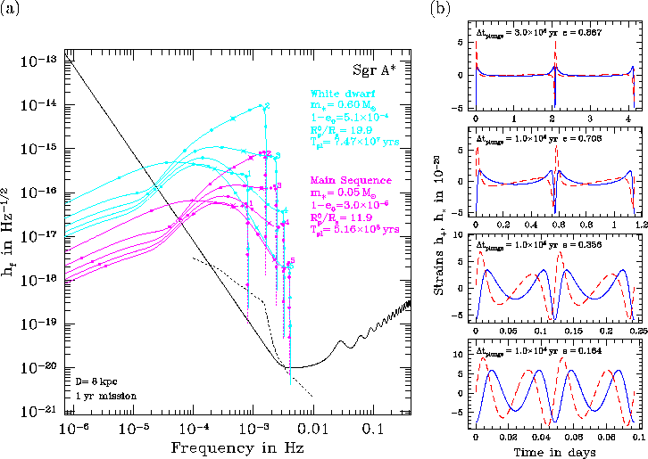
These orbital parameters are used to integrate the orbits of captured stars down to horizon crossing (Glampedakis et al., 2002) and compute the gravitational waves emitted (Pierro et al., 2001), as illustrated by Fig. 3.

Applying this computation to all capture events during some time interval, one determines the expected number of captured stars around Sgr A$^\ast$ that are emitting above any given LISA signal-to-noise ratio. Fig. 4 is the result of this procedure.

Figure 3: (a): Gravitational signal for two events from our Sgr A$^\ast$simulation, a WD and a low-mass MSS. We plot the amplitude vs frequency for the 5 first Fourier components of the quadrupolar radiation(Pierro et al., 2001). The crosses represent the position $1000$ years before plunge through the horizon. Other ticks show positions $10^6$, $10^5$, $10^4$, $100$, $10$, $1$ year, 1 month and 1 day before plunge. The dotted segments for the MSS correspond to a pericentre distance below tidal disruption radius. The solid black line is LISA's intrinsic noise( $\mathrm{SNR}=1$, Larson et al., 2000). The dashed line is an estimate of the confusion noise due to unresolved WD binaries in our Galaxy(Bender & Hils, 1997). (b): Waveforms ($+$ and $\times$ polarisations) at successive times during the orbital evolution of the MS star.

The most striking results concern MS stars. The predicted number of sources with SNR above 10 is of order 3-5 if one neglects tidal interactions until the stars enters the Roche zone ( $R_\mathrm{td}\simeq R_\ast (M_\mathrm{MBH}/M_\ast)^{1/3}$) and is considered destroyed. If one assumes pessimistically that all the energy of the tides (computed for a nearly parabolic orbit (McMillan et al., 1987)) is used to swell the star which is removed from the computation when the accumulated tidal energy amounts to 20% of its self-binding energy, one still gets of order 0.5-2 MSS sources with $\mathrm{SNR}\ge 10$.

Figure 4: Expected number of sources of gravitational waves at the Galactic centre. We show the number of objects predicted to produce a signal above a given signal-to-noise ratio ( $\mathrm{SNR}$). The orbital evolution of each captured star, as driven by emission of gravitational radiation around a non-spinning black hole, has been integrated down to plunge instability or tidal disruption(Glampedakis et al., 2002) and, at each time, we select the Fourier component of the quadrupolar radiation(Pierro et al., 2001) yielding the highest SNR. The upper curve for MS stars is obtained when tidal heating is neglected. The lower curve corresponds to a pessimistic estimate of the decrease in the number of sources due to tidal heating.

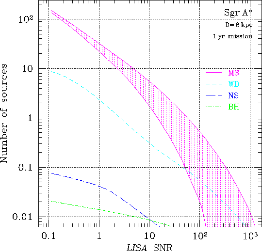Only very low mass MSSs contribute; more massive but less dense ones suffer from early tidal disruption. Hence, captured MSSs could only be detected at the Galactic centre, many $10^5$ years before plunge. All other sources are predicted to be compact remnants in galaxies at distances of a few hundreds of Mpc, during the last few months or years of inspiral.